#
#
Declarative Computation, Syntactic Sugar, and the Abstract Machine
The first kernel language that is explored and expanded upon in Van Roy and Haridi’s Concepts, Techniques, and Models expresses what the authors call the Declarative Computation Model.[3] Starting with Chapter 2, there is a large amount of material about this model in the book, and I hope to cover various aspects of it over the course of a few posts.
Leveraging the simplicity of the declarative model, in Chapter 2 we see up close how syntactic sugar enhances expressivity, and are treated to an in-depth look at the mechanics of the abstract machine, a device to reason about the execution of our code. I’ll dive a little bit into each in this post to lay the ground work for expanding the declarative model to include, for example, the primitives for “declarative concurrency.”
We aren’t given the best definition of declarative computation to start, only that it is “evaluating functions over partial data structures” and is sometimes known as “stateless programming.” The few examples here begin to flesh it out, but it is more interesting to grasp the basic mechanics here than to attempt to fill out a larger picture at this point.
Note: All quotes directly from CTM unless noted. Most code adapted from the text.
Syntactic Sugar
The declarative kernel language in the second chapter of CTM is very simple. There are few moving parts, and programs can be read and understood in a linear, predictable way. Nearly the entirety of the syntax of the language (excluding the value expression syntax) including everything we need to declare variables, assign values, execute statements, use conditionals, execute procedures, etc. fits in this small box:
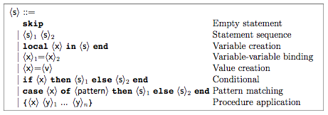
This predictability of the language comes at the cost of reduced expressiveness, but the idea is not to produce a perfect, industrial programming language. The point is to start from the basics, understand their formal foundations, and then progressively expand the expressive capabilities (and therefore the complexity of the underlying semantics) of your kernel language.
For our purposes, we need to know that:
local X in
end
declares an X variable. In other words it makes a variable X available to be bound to another variable or value within the scope of in…end. We also need to understand basic assignment:
X = 2In our data store X will now be forever bound to 2, and will be indistinguishable from its value. Finally, we have the concept of a procedure (proc). A procedure is a building block for a function in kernel languages. Take the following simple Simple proc form for example:
local Simple in
  Simple = proc {$ X ?Z}
    Z=1
  end
end
This proc will take a variable X and then regardless of its value, bind ?Z to 1. So:
local W in
  {Simple 1999 W}
end
Will end with 1 bound to W. Variables used within a proc do not have to be declared outside of it, but should be bound inside of it to ensure consistent behavior due to static scoping.
Using no syntactic shortcuts, here is how we we could define and use a Max procedure (as it is shown in the book), which given two inputs returns the one that is of greater numerical value. For example, {Max 3 5 X} should bind X to 5.
local Max in
  local A in
    local B in
      local C in
        Max = proc {$ X Y ?Z}
          local T in
            T=(X>=Y)
            if T then Z=X else Z=Y end
          end
        end
      A = 3
      B = 5
      {Max A B C}
      end
    end
  end
end
Using some shortcuts, the authors then show the following version. This can be unpacked to create the code above, or it can be used as it appears here:
local Max C in # declare variables Max (to hold proc) and C (to hold result)
  proc {Max X Y ?Z} # declare the proc (two inputs and one output), store it in Max
    if X>=Y then Z=X else Z=Y end # the Max algorithm
  end
  {Max 3 5 C} # call Max with 3 and 5, store the result in C
end
Syntactic Sugar is a code transformation which preserves semantics but eases use through clarification of intent. The following examples of syntactic sugar have been applied to the code in this example:
- Multiple variables declared per line (
local Mac C in) - ‘In-line’ values instead of variables (
proc {Max X Y ?z}) - Operations as expressions (
if X>=Y)
This illustration of syntactic sugar was an extremely effective way of understanding how the transformations the authors refer to actually work. It also showed me a way to keep programming languages simple: instead of changing semantics or introducing new operators, language authors can find more compact means of expressing the same semantics. The beauty of this reminds me of the tendency toward spare efficiency in good code. Code that can keep functions tight and packed with meaning by providing APIs that are composable is preferable because it easier to understand and reuse.
The Abstract Machine: Definitions
While syntactic sugar is one of the main mechanisms used to extend language functionality, the heart of understanding how the kernel languages operate is in how they execute in the abstract machine. As the authors say:
“We will define the kernel semantics as an operational semantics, i.e., it defines the meaning of the kernel language through its execution on an abstract machine.”
In other words, the abstract machine is the device, or the main metaphor, that is used to explain how the language works. An abstract machine executes the instructions that we give it in a predictable, repeatable way, and gives formal credence to our programmer’s intuition for how some basic programs work.
The abstract machine has a few components that need defining before we can examine how a relatively simple bit of code is executed.
Single assignment store ($\sigma$): a set of variables. Variables can be unbound (declared but not assigned a value) or bound (declared and assigned a value). Bound variables can be assigned the value of a number, a data structure, or another variable, but not rebound.
Environment ($E$): a mapping from variables to members of the single assignment store $\sigma$.
Semantic Statement ($ST$): a pair <$S$, $E$> where $S$ is a statement to be executed in environment $E$.
Execution State: The current state of the abstract machine.
Computation: The work done by the abstract machine:
“A single transition in a computation is called a computation step. A computation step is atomic, i.e., there are no visible intermediate states. It is as if the step is done ‘all at once.’”
With these definitions in place, we can proceed with program execution.
The Abstract Machine: Program Execution
An illustration of a small bit of declarative code (which actually does not have much syntactic sugar applied to it) as executed in the abstract machine can appear simple but still be quite instructive. The following piece of code and the accompanying prose that explains how it is executed in the abstract machine will illustrate how the declarative kernel language’s notion of static or lexical scope is calculated. Note the new Browse function, which displays the value given to the user, and that the <s> statement comments are referred to in the steps below.
local X in #<s> begin
  X = 1
  local X in #<s>1 begin
    X = 2
    { Browse X }
  end #<s>1 end
  { Browse X } # <s>2 begin/end
end #<s> end
Because the code and the kernel language in this state are so simple, you should be able to easily reason about it and predict how it will execute. As an exercise, answer the following question: What values will the Browse functions display, and in what order?
Luckily, we don’t have to just guess or work it out in our heads. The formalization of the abstract machine allows us to “calculate with environments,” or express its execution in a series of steps:
(1) $(ST, \sigma)$
The execution state is represented by a stack of semantic statements $ST$ and a value store $\sigma$.
(2) $([(\lt s \gt, \emptyset)], \emptyset)$
The initial execution state of our program in the abstract machine. $E$ has been replaced with $\lt s \gt$, a statement which represents the outermost $local$ statement in the program, and $\emptyset$, meaning there are not yet any mappings present. The value store has also been replaced with $\emptyset$ - it has no members.
(3) $([(\lt s \gt_1 \lt s \gt_2,\{X \rightarrow x\})], \{x = 1\})$
The outermost $local$ statement and $X = 1$ are executed. There is a sequential composition $\lt s \gt_1\lt s \gt_2$ remaining, the environment reflects that $X$ refers to the store variable $x$, and one binding ($x=1$) is added to $\sigma$.
(4) $([(\lt s \gt_1, \{X \rightarrow x\}), (\lt s \gt_2,\{X \rightarrow x\})], \{x = 1\})$
After executing the sequential composition we see that each statement ends up with its own environment; they are now on the execution stack. We will sequentially execute each statement next.
(5) $([(X=2 \{Browse \space X\}, \{X \rightarrow x’\}), (\lt s \gt_2,\{X \rightarrow x\})], \{x’, x = 1\})$
Executing $\lt s \gt_1$ binds a new variable $x’$ and calculates a new environment. This has a clear semantic specification; given an initial $E$ of $\{X \rightarrow x\}$, adding $\{X \rightarrow x’\}$ to it will yield $\{X \rightarrow x’\}$. The second mapping of $X$ overrides the first.
(6) $([(\{Browse \space X\}, \{X \rightarrow x’\}), (\{Browse \space X\}, \{X \rightarrow x\})], \{x’ = 2, x = 1\})$
$\lt s \gt_2$ is a $Browse$ statement, and $X = 2$ is bound. From this we can tell that we will see $Browse$ run twice - the first will show 2, and the second will show 1.
As demonstrated, the programmer’s intuition for scope can be reduced to a mechanical calculation. Awesome.
Conclusions
Most of us spend our time using programming languages which are considerably more expressive and complex than the declarative kernel language. The power of the kernel language approach is in its ability to illustrate how complexity and expressiveness can be derived from simple tools. As more elements are added to the language, the rules involved in translating the results from the computation steps in the abstract machine will also become more complex.
It’s an interesting exercise to consider how the programming language constructs you rely on could be composed of smaller, more atomic elements. Are all of the reducible? Working on a language like Ruby would be quite different than trying to reduce JavaScript or Scheme. Other paradigms for teaching computation from the ground up, including the interpreter approach championed by Friedman and Sussman advocate extending interpreters for smaller languages in order to run more complex ones. [1][2] This is an equally compelling approach that I intend to investigate in the future.
Now that we have seen how to define and execute a small language, we can begin to extend it. The variables in the Single Assignment Store have interesting properties that the authors leverage for various purposes, and before long a useful, beautiful language emerges.
Works Cited
[1] Harold Abelson, Gerald Jay Sussman, and Julie Sussman. Structure and Interpretation of Computer Programs, Second Edition. The MIT Press, Cambridge, Mass, 1996.
[2] Friedman and Wand. Essentials of Programming Languages. MIT Press, hardcover, ISBN-10: 0-262-206279-8, April 2008
[3] Van Roy and Haridi. Concepts, Techniques, and Models of Computer Programming MIT Press, hardcover, ISBN 0-262-22069-5, March 2004